Introduction
https://github.com/rfordatascience/tidytuesday/tree/master/data/2019/2019-01-22
From Github Readme: >Data Info > >Data comes from The Vera Institute GitHub. The raw dataset was >taken from their GitHub - it is in a wide format and if you are keen on really flexing your data munging skills it is a >worthy adversary! The truly raw data is seen >here. My full code >to reproduce the summary level datasets seen below can be found here, you can adapt this minorly to get >more data from the original wide dataset.
Loading Libraries
library(tidyverse)
library(maps)
library(viridis)
Read in Data
# Setting the root in one place so that I don't have to necessarily repeat the path
repo_root <- "https://raw.githubusercontent.com/rfordatascience/tidytuesday/master/data/2019/2019-01-22"

# This might take ~30s due to the volume of data
raw_data <- read_csv(glue::glue("{repo_root}/incarceration_trends.csv"))
pretrial_population <- read_csv(glue::glue("{repo_root}/pretrial_population.csv"))
pretrial_summary <- read_csv(glue::glue("{repo_root}/pretrial_summary.csv"))
prison_population <- read_csv(glue::glue("{repo_root}/prison_population.csv"))
prison_summary <- read_csv(glue::glue("{repo_root}/prison_summary.csv"))
Supplementary Data
state_name_to_abbrev <- data.frame(
  abbrev = state.abb,
  name = tolower(state.name)
)

county_xref <- raw_data %>%
  select(fips, state, county_name) %>%
  distinct() %>%
  inner_join(state_name_to_abbrev, by = c("state" = "abbrev")) %>%
  inner_join(maps::county.fips, by = "fips") %>%
  tidyr::separate(polyname, c("state","county"), ",") %>%
  select(-name)
## Warning: Column `state`/`abbrev` joining character vector and factor,
## coercing into character vector# Mapping Data
states <- map_data("state") %>%
inner_join(state_name_to_abbrev, by = c("region" = "name"))## Warning: Column `region`/`name` joining character vector and factor,
## coercing into character vectorcounties <- map_data("county") %>%
inner_join(state_name_to_abbrev, by = c("region" = "name")) %>%
left_join(county_xref, by = c("region" = "state", "subregion" = "county"))## Warning: Column `region`/`name` joining character vector and factor,
## coercing into character vectorData Munging
prison_population <-
  prison_population %>%
  mutate(pop_category_group = case_when(pop_category %in% c("Asian", "Black", "Latino", "Native American", "White", "Other") ~ "Ethnicity",
                                        pop_category %in% c("Female", "Male") ~ "Gender",
                                        pop_category == "Total" ~ "Total",
                                        TRUE ~ "Other")
         )
## Warning: package 'bindrcpp' was built under R version 3.4.4prison_pop_clean <- prison_population %>%
filter(between(year, 1990, 2015))# State Data ----
state_prison_pop <- prison_pop_clean %>%
group_by(year, state) %>%
filter(pop_category_group == "Total") %>%
summarise(population = sum(population, na.rm = TRUE),
prison_population = sum(prison_population, na.rm = TRUE)) %>%
mutate(prison_pop_per1k = prison_population / (population / 1000))
low_reporting_states <- state_prison_pop %>%
group_by(state) %>%
summarise(data_count = sum(prison_population > 0)) %>%
filter(data_count < 24) %>%
arrange(data_count)
state_prison_pop_median <- state_prison_pop %>%
filter(!(state %in% low_reporting_states$state)) %>%
group_by(state) %>%
summarise(median_rate = median(prison_pop_per1k))
# County Data ----
county_prison_pop <- prison_pop_clean %>%
group_by(year, state, county_name) %>%
filter(pop_category_group == "Total") %>%
summarise(population = sum(population, na.rm = TRUE),
prison_population = sum(prison_population, na.rm = TRUE)) %>%
mutate(prison_pop_per1k = prison_population / (population / 1000))
county_prison_pop_median <- county_prison_pop %>%
filter(!(state %in% low_reporting_states$state)) %>%
group_by(state, county_name) %>%
summarise(median_rate = median(prison_pop_per1k)) Exploration
Let’s start with the prison population.
# Let's Explore the different variables

prison_population %>% group_by(pop_category_group) %>% count()
## # A tibble: 3 x 2
## # Groups: pop_category_group [3]
## pop_category_group n
## <chr> <int>
## 1 Ethnicity 885198
## 2 Gender 295066
## 3 Total 147533Data Validation
- Total Population reporting switched from
Black, White, Other->Asian, Black, White, Latino, Native Americanin 1990- Based on the dramatic drop in
Whitecounts, manyLatino,Native American, and `Asian people we’re miscategorized prior to 1990
- Based on the dramatic drop in
- Prison Populations were reported differently by Ethnicity.
- Prison Populations are recorded between 1983 and 2015
- It appears that
Latinowas recorded in prison populations starting in 1983
Therefore, we should restrict analysis from 1990 to 2015
Many States (17) don’t have prison population data for all years in the analysis
Reporting of Ethnicity Changed in 1990
prison_population %>%
  #filter(complete.cases(.)) %>%
  group_by(pop_category, year) %>%
  filter(pop_category_group == "Ethnicity") %>%
  summarise(population = sum(population, na.rm = TRUE),
            prison_population = sum(prison_population, na.rm = TRUE)) %>%
  arrange(year) %>%
  ggplot(aes(x = year, y = population, color = pop_category)) +
  geom_line() +
  labs(title = "Population by Ethnicity",
       subtitle = "Reporting Changed in 1990",
       x = "Year",
       y = "Total Population") +
  scale_y_continuous(label = scales::comma) +
  theme_light()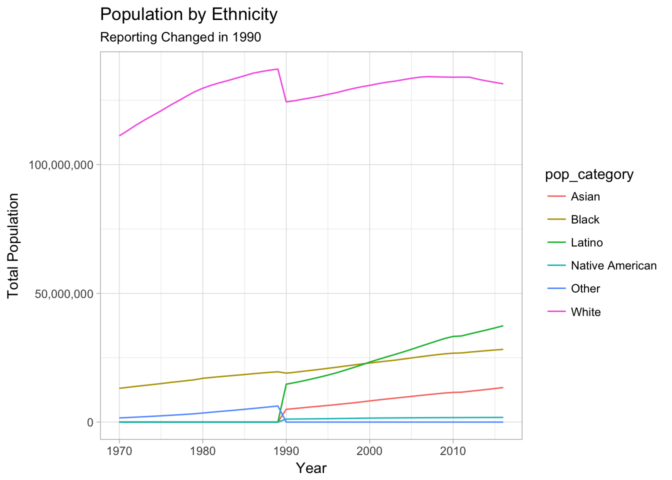
prison_population %>%
  #filter(complete.cases(.)) %>%
  group_by(pop_category, year) %>%
  filter(pop_category_group == "Ethnicity") %>%
  summarise(population = sum(population, na.rm = TRUE),
            prison_population = sum(prison_population, na.rm = TRUE)) %>%
  arrange(year) %>%
  ggplot(aes(x = year, y = prison_population, color = pop_category)) +
  geom_line() +
  labs(title = "Prison Population by Ethnicity",
       subtitle = "Prison Pop Reporting Covers 1983 to 2015",
       x = "Year",
       y = "Prison Population") +
  scale_y_continuous(label = scales::comma) +
  theme_light()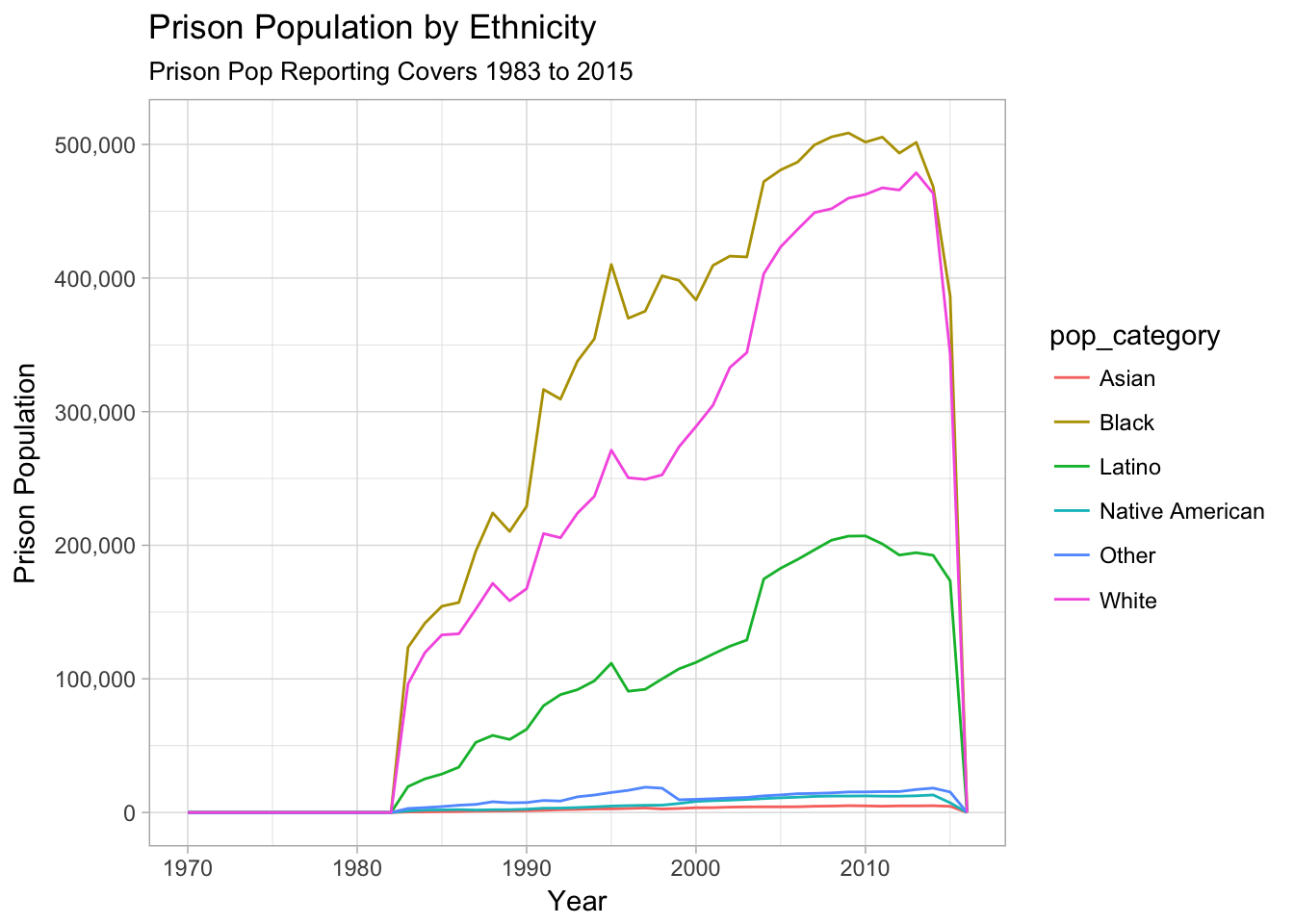
Some States have Spotty Reporting
low_reporting_states## # A tibble: 17 x 2
## state data_count
## <chr> <int>
## 1 AK 0
## 2 AR 0
## 3 CT 0
## 4 DC 0
## 5 DE 0
## 6 ID 0
## 7 KS 0
## 8 MT 0
## 9 NM 0
## 10 RI 0
## 11 VT 0
## 12 MA 8
## 13 LA 10
## 14 WY 10
## 15 IN 14
## 16 AZ 16
## 17 NV 22Incarceration Rate by State
state_prison_pop_median %>%
  top_n(10, median_rate) %>%
  ggplot(aes(x = forcats::fct_reorder(state, median_rate), y = median_rate)) +
  geom_point(size = 3) +
  geom_linerange(aes(ymin = 0, ymax = median_rate), size = 2) +
  geom_label(aes(label = round(median_rate, 1)), nudge_y = .5) +
  labs(title = "Top 10 States by Median Incarceration Rate",
       subtitle = "1990 to 2015 | 25 Years | 17 of 50 States Excluded for Missing Data",
       x = "State", y = "Median Incarceration Rate (1990 - 2015)") +
coord_flip() 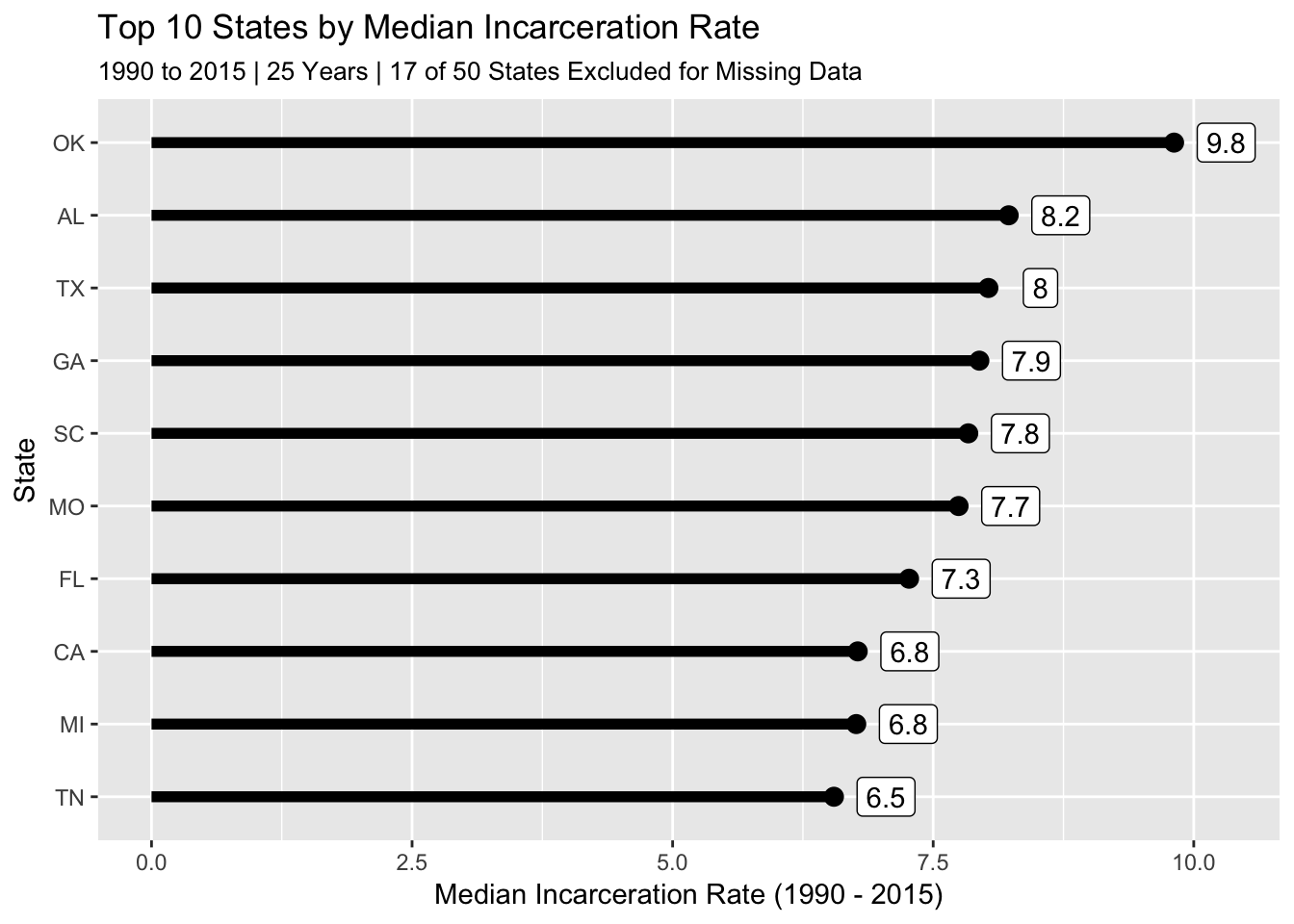
states %>%
  filter(!(abbrev %in% low_reporting_states$state)) %>%
  left_join(state_prison_pop_median, by = c("abbrev" = "state")) %>%
  ggplot() +
  geom_polygon(aes(x = long, y = lat, fill = median_rate , group = group), color = "black") +
  scale_fill_continuous(na.value = "#FFFFFF",low = "white", high = "darkblue") +
  coord_fixed(1.3) +
  guides(fill=FALSE) +
  labs(title = "Map of Median Incarceration Rates",
       subtitle = "Missing States have no data | Gradiant from Low (Lightest) to High (Darkest)") +
  theme_void()# do this to leave off the color legend
## Warning: Column `abbrev`/`state` joining factor and character vector,
## coercing into character vector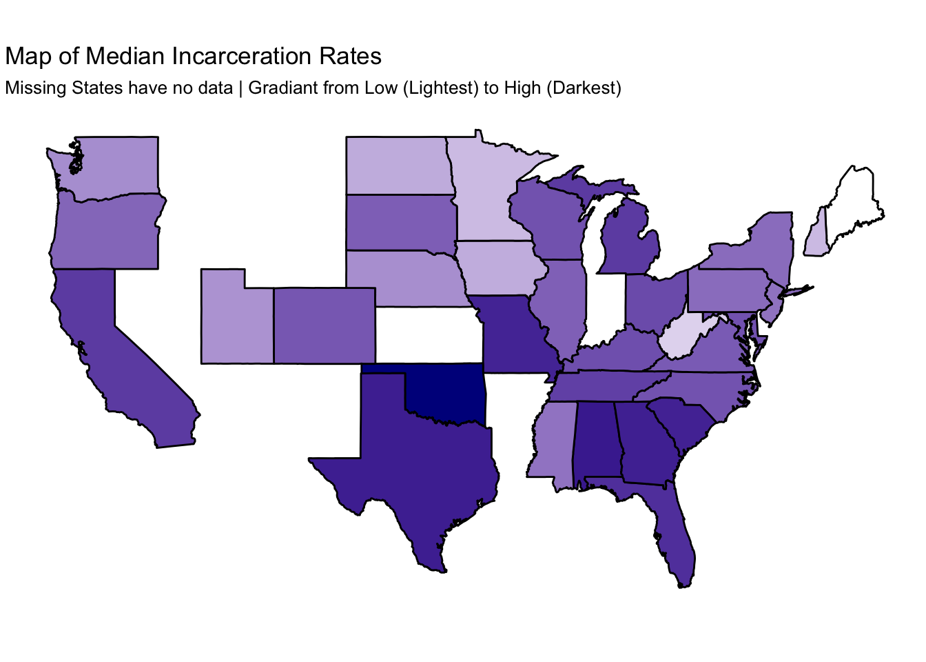
filter_county_prison_pop_median <-
  county_prison_pop_median %>%
  ungroup() %>%
  mutate(median_rate_ntile = ntile(median_rate, 1000)) %>%
  filter(between(median_rate_ntile, 2,998)) #%>%

# All Counties
counties %>%
  filter(!(abbrev %in% low_reporting_states$state)) %>%
  left_join(filter_county_prison_pop_median, by = c("abbrev" = "state", "county_name")) %>%
  ggplot() +
  geom_polygon(aes(x = long, y = lat, group = group, fill = median_rate), color = "lightgray", size = .2)  +
  geom_polygon(data = states, aes(x = long, y = lat, group = group), color = "black", alpha = 0, size = .1) +
  scale_fill_continuous(na.value = "#FFFFFF",low = "white", high = "darkblue") +
  coord_fixed(1.3) +
  guides(fill=FALSE) +
  labs(title = "Map of Median Incarceration Rates by County",
       subtitle = "Missing Counties / States have no data | Gradiant from Low (Lightest) to High (Darkest)") +
  coord_map() +
  theme_void()
## Warning: Column `abbrev`/`state` joining factor and character vector,
## coercing into character vector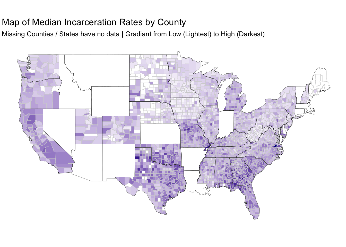
# Top Counties
counties %>%
  filter(!(abbrev %in% low_reporting_states$state)) %>%
  left_join(top_n(filter_county_prison_pop_median,500), by = c("abbrev" = "state", "county_name")) %>%
  ggplot() +
  geom_polygon(aes(x = long, y = lat, group = group, fill = median_rate), color = "lightgray", size = .2)  +
  geom_polygon(data = states, aes(x = long, y = lat, group = group), color = "black", alpha = 0, size = .1) +
  scale_fill_continuous(na.value = "#FFFFFF",low = "white", high = "darkblue") +
  coord_fixed(1.3) +
  guides(fill=FALSE) +
  labs(title = "Map of Median Incarceration Rates by County: Top 500",
       subtitle = "Missing Counties / States have no data | Gradiant from Low (Lightest) to High (Darkest)") +
  coord_map() +
  theme_void()
## Selecting by median_rate_ntile## Warning: Column `abbrev`/`state` joining factor and character vector,
## coercing into character vector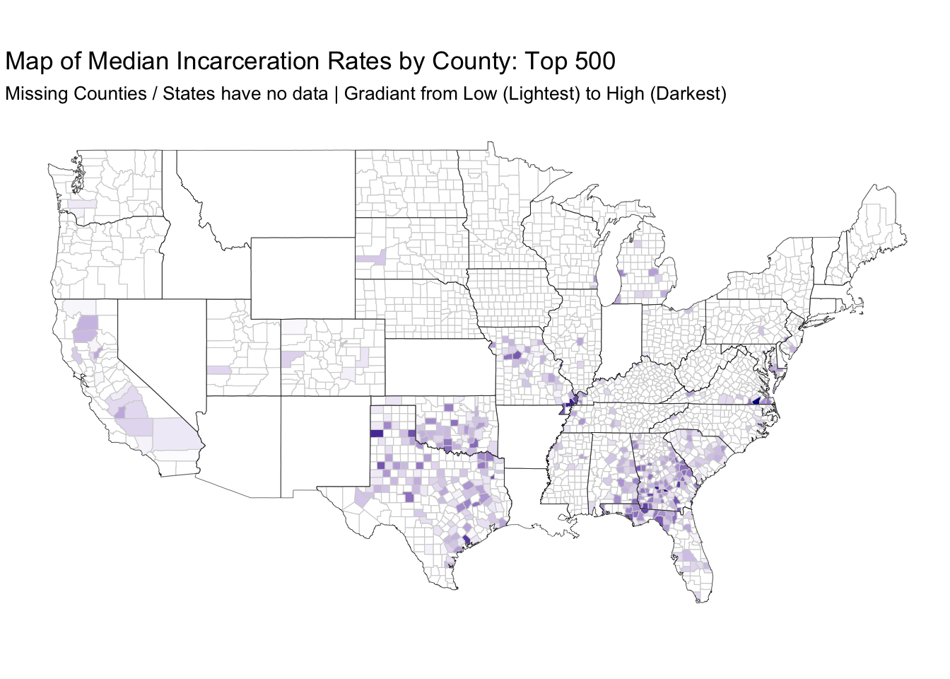
Twitter
Google+
Facebook
Reddit
LinkedIn
StumbleUpon
Pinterest
Email